
Model development is the third phase of the ML lifecycle, where we build the ML models for our problems and evaluate their performances.
Select models
This part focuses on mapping our ML problems to appropriate ML algorithms. Knowledge of common ML tasks and the typical approaches to solving them is essential in this process.
When selecting a model, we need to consider:
- Model's performance is measured by metrics such as accuracy, F1, log loss, etc.
- How much data the model needs to run
- How much computing and time the model needs to do both training and inference
- Model interpretability
Tips to select models
- Avoid the state-of-the-art models
- Start with the simplest models. E.g., a simple model or complex model with ready-made implementation
- Avoid human biases in model selection
- Take into account the incoming new data. E.g., evaluate the model learning ability by using learning curve (opens in a new tab)
- Evaluate trade-offs. E.g., false positives vs. false negatives, model accuracy vs. computing resources, etc.
- Understand the model's assumptions
- Independent and identically distributed (opens in a new tab): in ANN, all examples are independently drawn from the same joint distribution
- Smoothness: supervised ML method assumes that if an input X produces an output Y, then an input close to X would produce an output proportionally close to Y
- Boundaries: a linear classifier assumes that decision boundaries are linear
Ensembles
In the beginning, we start with one model. Later, we might want to improve the system by using an ensemble of several models to make predictions. Each model in the ensemble is called a base learner.
Bagging (Boostrap aggregating)
- Bootstrap data: randomly sample data records to create N sets of data. The records can be overlapped
- Use N identical models to train on those N sets of data
- Final prediction is the average predictions of N models
Boosting
- Train model 1 on the dataset, take out the wrong predicted data
- Train model 2 on the original dataset and the wrong predicted data in the previous step
- Continue training like that until model N
- Final prediction is the weighted predictions of each model
Stacking
- Split data into two parts, P1 and P2
- Train N base models which are different in architecture on P1
- Perform inference for these N trained models on P2 to generate a set of new features
- Train 1 meta-model on the new features in the previous step. The final prediction is the meta-model's prediction
Below is the table to compare those three ensembles.
| Bagging | Boosting | Stacking | |
|---|---|---|---|
| Data sampling | Use bootstrap to create N datasets; records can be overlapped (sampling with replacement) | The later model's data is the original data + previous model's wrong-predicted data | Split data into two parts, one is for N base models, the other is for meta-model (or generalizer) |
| Architecture | N identical models | N identical models | N different models + 1 meta-model |
| Application | Decrease high variance of N complex models | Decrease high bias of N simple models | Improve model performance |
| Example | Random forest use N decision trees | Use N decision trees with low depth (to have low complexity model -> high bias) | Use three base models (decision tree, kNN, SVM) + 1 meta-model (ANN) |
Note:
- High bias/high variance is the trade-off when training a model, not a model's characteristic
- Low complexity model or high bias: under fitted, prediction is biased
- High complexity model or high variance: overfitted, prediction fluctuates
Train models
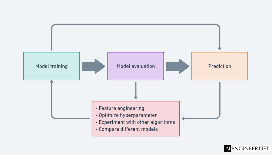
Training, tuning, and evaluation are iterative processes.
Split data
Firstly, we need to split the data to ensure the division between the training and evaluation efforts. A common strategy is to split data into training, validation, and testing subsets with a common ratio of 80:10:10 or 75:15:15.
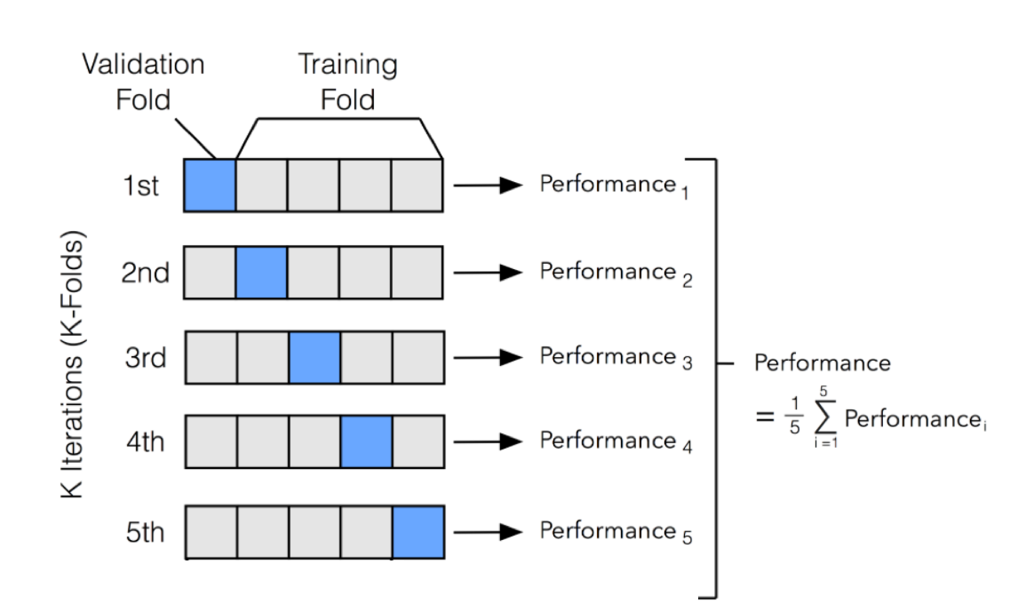
Cross-validation is another technique to compare multiple models' performance. The goal is to choose the model that will eventually perform the best in production.
k-fold cross-validation is a common validation method. In k-fold cross-validation, you split the input data into k subsets of data, so-called folds. You train your models on all but one (k-1) of the subsets and then evaluate them on the subset not used for training. This process is repeated k times, with a different subset reserved for evaluation (and excluded from training).
If you have a small dataset, consider leave-one-out cross-validation (LOOCV), k-fold cross-validation where k is set to the number of examples in the dataset. Learn more about LOOCV here (opens in a new tab).
If you have imbalanced data, consider Stratified k-fold cross-validation, where the distribution of classes in each fold is kept. Learn more here (opens in a new tab).
Cross-validation techniques will increase the computational power needed for your training.
For more details about data sampling, please refer to the post Data Engineering - Sampling in this The Ultimate Machine Learning System topic.
Optimize hyperparameters
To find the suitable model, we usually have to tune our model after training by performing additional feature engineering, experimenting with new algorithms, etc., by training and evaluating multiple models that use different data setups and algorithms. This model tuning also involves modifying the model's hyperparameters.
Hyperparameters are settings that can be tuned before running a training job to control the behavior of an ML algorithm. They can have a significant impact on model training related to training time, model convergence, and model accuracy. Unlike model parameters derived from the training job, the values of hyperparameters do not change during the training.
There are different categories of hyperparameters, such as:
- Model hyperparameters: define the model itself. For example, attributes of a neural network architecture like filter size, pooling, stride, padding
- Optimizer hyperparameters: are related to how the model learns the patterns based on data and are used for a neural network model. For example, optimizers like gradient descent, stochastic gradient descent, Adam, Xavier initialization, He initialization, etc.
- Data hyperparameters: are related to the attributes of the data, often used when you don't have enough data or enough variation in data. For example, data augmentation techniques like cropping, resizing
Traditionally, this was done manually. Someone with domain experience related to that hyperparameter and the use case would manually select the hyperparameters based on their intuition and experience. Then they would train the model and score it on the validation data. This process would be repeated repeatedly until satisfactory results are achieved. As a result, several other methods for hyperparameter tuning have been developed.
Alternatively, some tools offer automated hyperparameter tuning, which uses gradient descent, Bayesian optimization, and evolutionary algorithms to conduct a guided search for the best hyperparameter settings by running many training jobs on your dataset using the algorithm and ranges of hyperparameters that you specify. For example, Weights and Biases (opens in a new tab).
Experiment tracking and versioning
We experiment with different models with different hyperparameter configurations in the model development phase. It's important to keep track of all the experiments and artifacts, such as the loss curve, evaluation loss graph, logs, etc. This helps us compare different experiments to understand the effect of different changes in the model's performance to choose the best model.
Experiment tracking is tracking the progress and results of an experiment.
Versioning is the process of logging all the details of an experiment to recreate it later or compare it with other experiments.
Below is the list of some possible things we might want to track.
- Who run the experiment?
- Start time, end time
- Model configuration
- Feature names
- Hyperparameters: learning rate, learning rate schedule, gradient norms, weight decay, momentum, etc.
- Data: reference to training data, validation data, test data, feature distribution, statistics
- Speed of the trained model
- Number of steps per second
- Number of tokens processed per second
- Model performance
- Performance metrics: accuracy, F1, etc.
- Charts: loss curve, ROC, PR, confusion matrix, etc.
- System performance: memory/CPU/GPU utilization
- Full learned weights
- Summary of the trained model
Some tools to track experiments and versioning are Weights and Biases (opens in a new tab), DVC (opens in a new tab), mlflow (opens in a new tab), etc.
Debug models
Below is the list of things that might cause an ML model to fail.
- Theoretical constraints: the assumptions about the data and the features that the model uses are wrong
- Poor model implementation: forget to stop gradient updates during evaluation, etc.
- Poor choice of hyperparameters: different sets of hyperparameters give different results
- Data issues: data is collected unproperly, labels are wrong, features are processed wrongly, etc. For more details on data issues, please refer to the post Data Engineering - Data Issues in this The Ultimate Machine Learning System topic.
- Poor choice of features: too many or too few features
AutoML
We can use AutoML tools to automate preprocessing data, selecting models, tuning hyperparameters, and choosing the best model. For the comparison of AutoML libraries, please refer to this AutoML Libraries Comparision article (opens in a new tab).
Distributed training
It's common to train a model using a dataset that doesn't fit into memory, such as CT scans. In this case, we need algorithms for preprocessing, shuffling, and batching data out-of-memory and in parallel. This requires training ML models on multiple machines using multiple CPUs, GPUs, and TPUs.
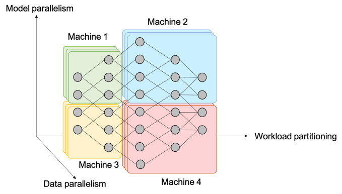
Data parallelism
The most common parallelization method is data parallelism: we split the dataset on multiple machines, train the model on them, and accumulate gradients.
Challenge 1: How to accurately and effectively accumulate gradients from different machines
In Synchronous stochastic gradient descent (SSGD), the model waits for all machines to produce their gradients. This causes the training to slow down, wasting time and resources.
In Asynchronous stochastic gradient descent (ASGD), the model updates weights using the gradient from each machine separately. This causes the gradient stateless issue when gradients from one machine have caused the weights to change before the gradients from other machines come in.
In theory, ASGD converges but requires more steps than SSGD. However, in practice, when gradient updates are sparse, most gradient updates only modify small fractions of the weights, the model converges similarly (opens in a new tab).
Challenge 2: Big batch size
The batch size can be huge when spreading the model on multiple machines. If a machine processes a batch size of 1000, 1000 machines process a batch size of 1M. Increasing the batch size past a certain point causes diminishing returns.
Model parallelism
Model parallelism splits different components of the model on different machines.
Challenge: parallel computing
If the model is a massive matrix and the matrix is split into two halves into two machines, these two halves might be executed in parallel. However, if the model is a neural network and the first layer is on machine one while the second layer is on machine 2, machine 2 must wait for machine 1 to finish.
To solve this, we can use the pipeline parallelism technique to make different components of a model on different machines run more in parallel. The idea is to break the computation of each machine into multiple parts. When machine 1 finishes its computation, it passes the output to machine two and continues with the next computation while machine 2 executes its computation on the output returned by machine 1. Each machine can run both forward pass and backward pass for one neural network component.
Many organizations use both data parallelism and model parallelism to better utilize their hardware. However, the setup to use both methods can require significant engineering effort.
Ending
This post covered the common steps when developing ML models: model selection and model training processes. The distributed training is usually handled by the ML infrastructure engineer or ML platform engineer. A data scientist doesn't necessarily need to know about it.